Understanding waste in Manufacturing:

SUSTAINABILITY has quickly become a core priority in modern manufacturing, driven by growing demand for products that are more eco-friendly and a lower impact on the environment. This is due to a new need within the manufacturing industry to be more environmentally conscious and uphold a higher responsibility on the impact that most of the manufacturing processes have.

In industrial production systems, particularly in energy- and resource-intensive sectors, waste manifest in various forms like material loss or energy consumption waste, which creates a necessity for companies to create digital solutions as a way to better understand waste in manufacturing processes by identifying and quantifying manageable elements that influence waste, enhance product quality and promotes a more profitable and sustainable operation.

The iron and steel industry faces these challenges constantly despite their advances in technology. The production of sponge iron (also known as direct reduced iron DRI) is famous for it's waste due to their nonlinear and highly complex thermochemical reactions that occur on a huge reactor under strict temperature and pressure conditions. As a result, monitoring and managing quality deviations and waste in real-time is a significant challenge. (AND also a key opportunity for data analysis and optimization modeling)

Thanks to the integration of advanced data analytics and machine learning techniques into manufacturing systems, it has become possible for thousands of sensors and sample data measurements to be processed for interpretation. In the context of sponge iron production, these tools allows to develop predictive models that link raw material quality, temperature and pressure sensor data within the direct reduction reactor, and the final product characteristics.

This enables a dynamic quality control loop where deviations can be anticipated and corrected before they turn into waste at the end of the manufacturing process.

This project explores how data-driven interpretations of complex processes can support two main objectives: Quality control and Quality prediction. These objectives are approached through the lens of simulated process data typically encountered in a sponge iron plant.

Throughout this project we will use the CRISP-DM methodology in order to generate predictive models that can be used to forecast waste generation by identifying patterns through control sensors within a direct reduction reactor, and information obtained from material samples taken before and after the process, starting with the understanding of business objectives and ending with the evaluation of the model, along with actionable insights on the data.

Within this project, we will explore the concept of manufacturing sustainability and how interpretations of analyses and models can be used to control waste production and predict waste generation. By leveraging data-driven approaches which manufacturers can then use to identify the sources of waste, optimize their production processes, and reduce their environmental footprint.

The broader goal of this project is to showcase how manufacturers can leverage statistical modeling and machine learning for identifying sources of waste, monitor quality indicators and improve the utilization of resources.

NOTE: All data within this project is simulated and does not reflect real operational or sample data commonly found within actual existing sponge iron manufacturing plant. The conclusions reached at the end of the project does not truly represent findings that could be applicable to a real sponge iron production plant.

STEP 1: Business Understanding

I. Quality control:
Quality control is an essential process within manufacturing that aims to identify and correct any defects or deviations from the ideal production process. This project is developed for the analysis of data from various quality control sensors for the purpose of identifying patterns of quality issues considering all elements involved in the manufacturing process.

By pinpointing the sources and timing of these deviations, interventions can be applied in real time in order to stabilize product quality and reduce unnecessary material and energy waste.

II. Quality prediction:
Quality prediction in manufacturing processes uses data and statistical modeling to forecast the quality of the final product based on the input variables and process parameters. The goal is to identify potential quality issues early in the production process, giving the manufacturer the opportunity of correcting the production before the generation of the final product.

In a sponge iron plant, this means forecasting final product characteristics (e.g., porosity, metallization, carbon content) from variables such as feed composition, reactor temperature, and pressure. Anticipating product quality enables proactive process adjustments that can prevent waste before it occurs.

For Key Performance Indicators (KPI) we'll take into consideration the value added to the manufacturing process when it's adapted to deal with waste production. The KPI's should promote a decrease in costs, an increase in profits, and a reduction of environmental impact. (As waste usually represent inefficient processes, low quality product or a combination of both)

STEP 2: Data Understanding

Data understanding involves all activities related to exploring the structure, content, and quality of the datasets involved in the problem. For this manufacturing project, the primary focus is to assess the usability of the sensor readings, material samples and production data that is collected across different stages of the sponge iron DRI process simultaneously.

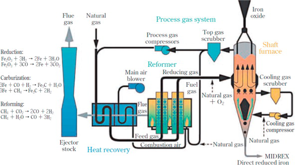
Before continuing the project, it's important to briefly introduce the underlying process. Sponge iron is a metallic product produced by the direct reduction of iron ore within a direct reduction reactor within a relatively controlled environment. Unlike blast furnaces, which uses coke (a type of solid fuel) as a reducing agent at lower temperatures. The reduction process involves using gases such as gases such as hydrogen (H₂) and carbon monoxide (CO).

Within the DR reactor the iron ore experiences several chemical and thermodynamic processes such as "Redox" reaction, "Gas-solid" reactions with reducing agents, and Heat transfer mechanisms encompass a highly complex manufacturing process with dozens of material inputs and highly sensitive reactor conditions, and external agents introduced during processing. Which is why understanding how these variables interact and influence each other is critical before applying any quality control or predictive models.

Before applying any type of data models for quality control or quality prediction, we'll first have to understand the scale and range of the data. In this case, the project will take into account the production volume, raw material data, sensors within the reactor and quality control records.

NOTE: Within this project we won't consider any data quality issues like anomalies or missing data as all data is generated specifically for this project.

The following are the main datasets included in this project:

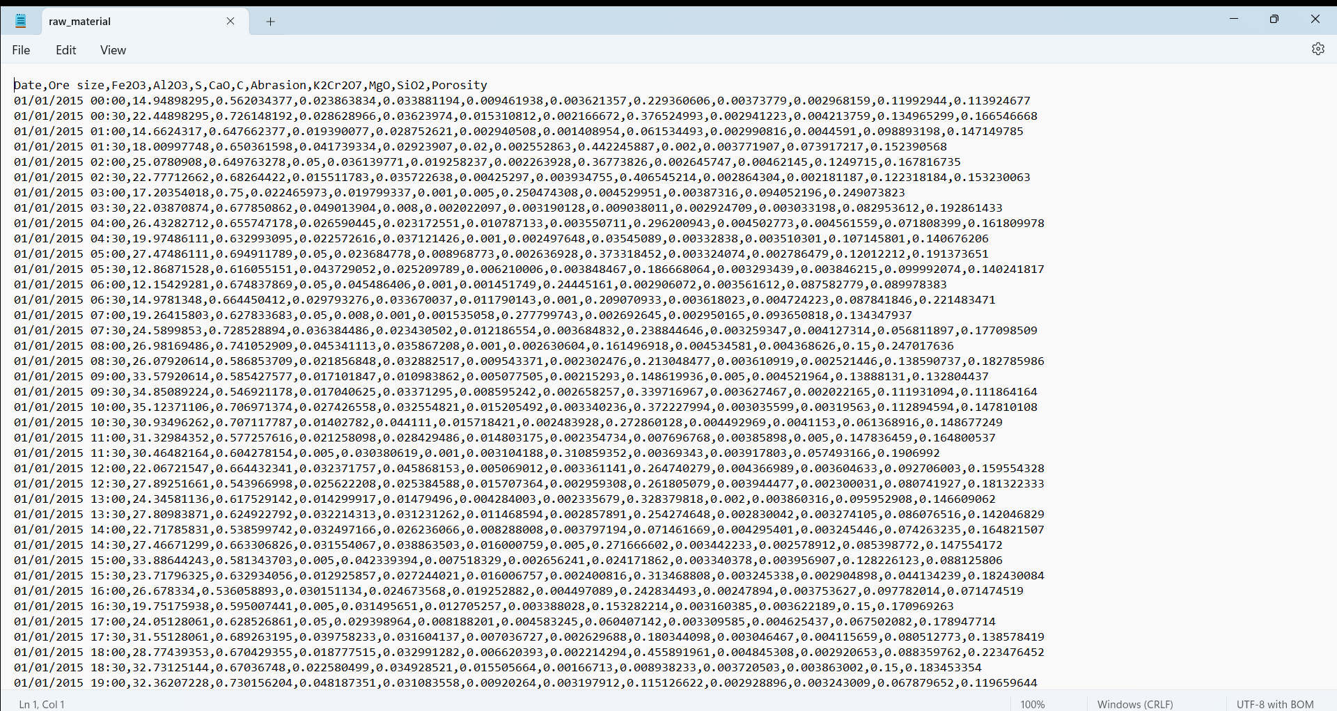
1. Raw material sample data: these variables represent the physical and chemical characteristics, dimensions and composition of iron ore before it is introduced into the direct reduction reactor. Which is why understanding these input features is essential, as they influence the quality of reduction and the formation of impurities in the final product.
+ Ore size (cm)
+ Iron oxide purity % (Fe₂ O₃)
+ Impurity 1 % (Al₂O₃)
+ Impurity 2 % (S)
+ Impurity 3 % (CaO)
+ Impurity 4 % (C)
+ Abrasion measure (mm³)
+ K₂Cr₂O₇ content
+ MgO content
+ SiO₂ content
+ Unit of Porosity % (Φ)

2. Reactor sensors: represent the internal environment of the direct reduction reactor which is monitored at different locations through the use of thermocouples and manometers in order to measure the temperature and pressure respectively. These sensors offer insights regarding the stability and consistency of the chemical reactions.
+ Temperature measurement 1 (C°)
+ Pressure measurement 1 (Pa)
+ Temperature measurement 2 (C°)
+ Pressure measurement 2 (Pa)
+ Temperature measurement 3 (C°)
+ Pressure measurement 3 (Pa)
+ Temperature measurement 4 (C°)
+ Pressure measurement 4 (Pa)
+ Temperature measurement 5 (C°)
+ Pressure measurement 5 (Pa)

The code resamples this data into 30-minute intervals and computes rolling averages in order to smooth the small fluctuations that naturally occur within the reactor as a way to simulate real industrial monitoring systems.

3. Agent flows: includes the injection of reagents, chemical binders and fluxes added within the direct reduction reactor for the purpose of chemically altering the iron pellets into sponge iron. Measured in flow rates.
+ Reagent 1 H₂ (L/min)
+ Reagent 2 CO (L/min)
+ Reagent 3 CH ₄ (L/min)
+ Binder 1 Al₂O₃ (kg/min)
+ Binder 2 4SiO₂ (kg/min)
+ Binder 3 C₆H₁₀O₅ (kg/min)
+ Binder 4 C₁₂H ₂₂O₁₁ (kg/min)
+ Flux 1 CaCO₃ (L/min)
+ Flux 2 CaMgCO₃
+ Flux 3 SiO₂

Agent flows are a very important element to the direct reduction process since every type of chemical component has a function to the overall state of the final product.

For example, the Reagents (or reducing gas) react with the iron oxide (FeO) in the direct reduction process to produce sponge iron (Fe), while Binders are powders that are then added to hold fibers together and create a cohesive structure of the iron pellets, and finally Fluxes serve to promote the chemical reactions that happen under certain environmental conditions.

Understanding the function of these compounds is key to linking their flow behavior to process outcomes. For example, variations in H₂ flow may affect metallization, while inconsistencies in binder composition could increase abrasion or waste powder generation.

4. DRI sample data: serve as a way to analyze the distribution between the final product and the waste generated after the Direct Reduction process, as well as the quality of the DRI final product which is measured by the types of impurities commonly found within the iron ore.
+ DRI pellet %
+ Pellet size (cm)
+ DRI purity % (Fe)
+ Impurity 1 % (S)
+ Impurity 2 % (C)
+ Metallization %
+ Slag %
+ Waste powder %
+ Unit of Porosity % (Φ)

STEP 3: Data Preparation

Now that all data has been collected and preprocessed, we can observe that each dataset originates from a different sampling point within the direct reduction process. This reflects how actual slow industrial processes function, where data is generated asynchronously from multiple stages of production. For this reason, the model has to adapt the information by linking the output data with the multiple different sources of input data.

This allows the model to trace the transformation for every single pellet batch of iron ore throughout the entire DRI production cycle, by aligning the datasets at their relevant time-steps. In a typical DRI process, a complete transformation - from raw pellet input to reduced iron output - takes approximately 9 hours.

# Python CODE: Aggregation of data
In the code, this logic is applied directly to the df_raw_material dataframe by subtracting 9 hours from the timestamp. This aligns the raw material features with the corresponding DRI output for each batch.

try:
     df_raw_material['Date'] = pd.to_datetime(df_raw_material['Date'], format='%d/%m/%Y %H:%M')
except ValueError as e:
     df_raw_material['Date'] = pd.to_datetime(df_raw_material['Date'], format='mixed')
df_raw_material['Date'] = df_raw_material['Date'] - pd.Timedelta(hours=9)

Next, we consider the sensor data collected from within the direct reduction (DR) reactor. These variables include pressure and temperature readings from various reactor zones, recorded at high frequency (every 2 minutes). To reduce granularity and enhance interpretability, these measurements are resampled to 30 minute intervals, calculating the mean and standard deviation as a way to capture the central tendencies but also it's operational variability.

The final quality metrics observed in the DRI samples at time t are influenced by the raw material and operating conditions that occured at time t - 9 hours. Consequently, each of the four datasets introduced in the data understanding phase must undergo a temporal adjustment to reflect their role in this 9 hour transformation window.

For example, if a DRI pellet is sampled at around 4:00 PM, the raw material properties responsible for its formation would have been recorded at around 7:00 AM. In order to link both of these datasets, the data preparation phase has to shift the timestamp of the raw material dataset back by 9 hours. This adjustment allows us to construct a causal link between the input material data and the output DRI pellet quality data.

# Python CODE: Rolling window CODE

try: resampled_df = df_reactor_sensor.resample('30T').agg({
                              'Temperature 1': ['mean', 'std'], 'Pressure 1': ['mean', 'std'],
                              'Temperature 2': ['mean', 'std'], 'Pressure 2': ['mean', 'std'],
                              'Temperature 3': ['mean', 'std'], 'Pressure 3': ['mean', 'std'],
                              'Temperature 4': ['mean', 'std'], 'Pressure 4': ['mean', 'std'],
                              'Temperature 5': ['mean', 'std'], 'Pressure 5': ['mean', 'std']})
resampled_df.reset_index(inplace=True) However, aligning the sensor data with the DRI output is more complex. Because the reactor continuously processes material over the 9-hour period, the relevant sensor readings are those observed throughout the entire time window leading up to the sampling of the DRI.

To account for this, a rolling window technique is applied across the sensor time series. The rolling average and rolling standard deviation over a 9-hour window are computed to represent the cumulative effect of reactor conditions on each pellet batch.

df_reactor_sensor = df_reactor_sensor.rolling("9H").mean()
df_reactor_sensor = df_reactor_sensor.iloc[18:]

This technique is extended to the agent flow dataset as well. Similar to the sensors, the composition and quantity of reducing gases, binders and fluxes vary over time and influence the chemical reactions inside the reactor. Applying a rolling window to this dataset allows us to compute the average behaviours and fluctuations of key components over the same 9-hour period.

By using time-shifting and rolling window aggregation, we transform the original asynchronous datasets into a unified, temporally aligned dataset. Each row in the final version of the merged DataFrame now represents the same iron ore throughout the entire process linking: the raw material characteristics, the reactor's internal state during the pellet's transformation, the chemical agents involved, and the final DRI quality outcomes.

Thanks to aggregating the reactor data, we ensure that the input features and target variables reflect true process dependencies, thereby improving the relevance and accuracy of our quality prediction and waste estimation models. This also prevents any alignment of mismatched observations.

STEP 4: Data Exploration and Visualization

Now that the data from all sources are completely aligned it is time to apply data exploration and visualization techniques in order to understand the data's characteristics, uncover potential patterns, and make informed decisions about which variables are relevant for the modeling phase.

Due to the fact that we are handling a great number of independent variables (52) it is important for us to first examine dimensionality problems that might surface when building our model. This is done because Dimensionality reduction improves the interpretability, stability, computational efficiency and performance of statistical models and forecasting algorithms.

Dimensionality problems arise when multiple variables are highly correlated, which means that they carry redundant information. This redundancy can inflate the dimensionality of the dataset without providing new insights. Within this project, we will try out two different methods of dimensionality reduction and compare the performance of the model, as a way to objectively compare which method offers higher value to the end result.

The methods that we'll try out during this project will be Reverse Stepwise Regression and Principal Component Analysis (PCA) which both require an in-depth analysis of the relationships between independent variables as a way to determine which variables offer redundancy within the dataset. In this project, we will not only apply basic Pearson correlation metrics but also prove if there are non-linear relationships between the variables using Spearman's rank correlation coefficient.

Note: Reverse Stepwise Regression and PCA will help in understanding which variables impact the most in waste generation (Quality Control) and enable the creation of more accurate models that forecast the amount of waste produced (Quality prediction).

Pearson's correlation matrix measures the linear relationship between two continuous variables, which in the case of our dataset, it is applicable to all prepared data. Pearson's correlation is commonly used when analyzing relationships between variables with continuous data, assuming that the data is normally distributed and that the relationship between all variables is linear.

import pandas as pd import seaborn as sns import openpyxl import matplotlib.pyplot as plt from pyscript import display df_1 = pd.read_excel('correlation_matrices.xlsx', sheet_name="Pearson Correlation", header=0, index_col=0) fig1, ax1 = plt.subplots() sns.heatmap(df_1, annot=False, cmap="Blues", ax=ax1, xticklabels=False, yticklabels=False) plt.title("Pearson correlation (DRI process)") display(fig1, target="pearson_heatmap")

Spearman's correlation matrix measures instead the strength and direction of a monotonic relationship between two variables. Pearson's correlation coefficient does not assume linearity between the variables, nor does it assume that the data is normally distributed, which is particularly helpful if there are exponential, logarithmic or even polynomial relationships between two variables.

import pandas as pd import seaborn as sns import openpyxl import matplotlib.pyplot as plt from pyscript import display df_2 = pd.read_excel('correlation_matrices.xlsx', sheet_name="Spearman Correlation", header=0, index_col=0) fig2, ax2 = plt.subplots() sns.heatmap(df_2, annot=False, cmap="Greens", ax=ax2, xticklabels=False, yticklabels=False) plt.title("Spearman correlation (DRI process)") display(fig2, target="spearman_heatmap")

STEP 5: Feature Engineering

For "Reverse Stepwise Regression", the goal is to remove the least significant predictor (based on p-value) at each step, by fitting the complete dataset into a model to the data, evaluate its performance and then slowly remove all predictors that have the least significance until the performance of the model reaches it's peak.

On the other hand, Principal Component Analysis (PCA) is built by transforming the dataset into principal components, through the use of Eigendecomposition which decomposes the group of dependent variables into their respective eigenvectors and eigenvalues. PCA then selects the top Principal components by picking out eigenvectors based on their corresponding eigenvalues.

For both cases, we will have to preprocess the dataset by scaling all data equally. This is done because most of the independent variables don't share the same metrics (Pressures, Temperatures, Percentages, Measurements, etc.). There are many different scaling methods from the sklearn.preprocessing library like StandardScaler, MinMaxScaler, RobustScaler, etc. that have the same goal of standardizing data.

# Python CODE: MinMaxScaling
After applying both "Shapiro-Wilk" and "Kolmogorov-Smirnov" tests for normality and goodness of fit. We can determine that none of the independent variables follow a normal distribution which pushes us to use the MinMaxScaler as it's particularly effective when the data is not normally distributed, by applying a scaling method that doesn't assume any distribution and scales the data to a range of [-1, 1], preserving the original non-normal distribution.
Note: MinMaxScaler applies a uniform scaling by subtracting the minimum value and dividing by the range of the dataset.

from sklearn.preprocessing import MinMaxScaler
scaler = MinMaxScaler()
independent_variables = final_variables.iloc[:, 1:].copy()
independent_variables.columns = independent_variables.columns.astype(str)
independent_variables = scaler.fit_transform(independent_variables)

# Python CODE: Principal Component Analysis (PCA)
In scikit-learn, PCA is implemented as a transformer object that learns components in its fit() function, which computes the covariance matrix, handles the eigendecomposition on the covariance matrix and then generates the principal components.

from sklearn.decomposition import PCA
pca_dri = PCA()
pca_dri.fit(independent_variables)
principal_components = pca_dri.transform(independent_variables)
selected_components = principal_components[:, :6]

The PCA components will be later fed into a General Additive Model (GAM) regression model that will consider the complexity of the relationships between the independent and dependent variables, as well as offer an in-depth statistical analysis of the entire process.

Thanks to the explained_variance_ratio_ function within sklearn.decomposition we can measure the percentages of variance explained by each of generated principal components. By calculating the accumulated sum of the ratios we can determine that the total variance of the first 6 PCA components reach a variance of 92.39%. (If we handle 5 Components the percentage is 87.97% and if we handle 7 PCA components the variance reaches 93.61%)

Note: If we use 14 or more components, the explained_variance_ratio_ is 1.0 indicating that we’ve captured 100% of the variance in the dataset.

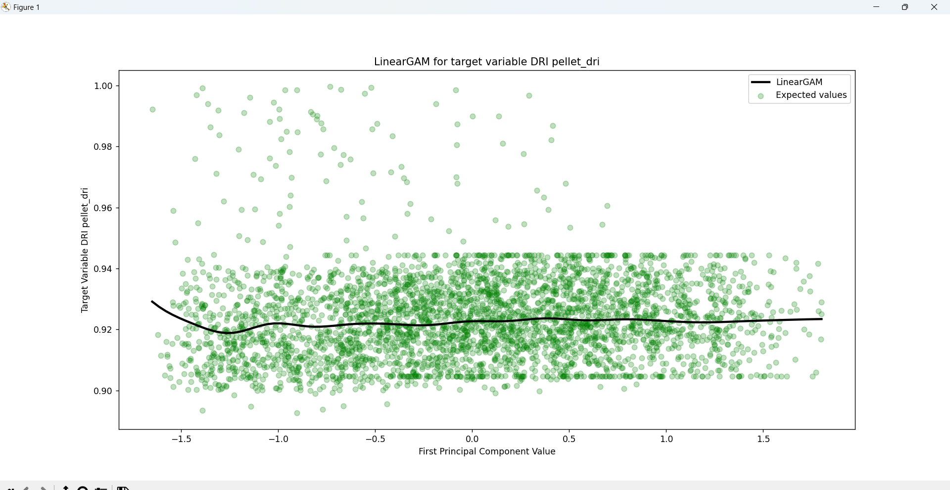
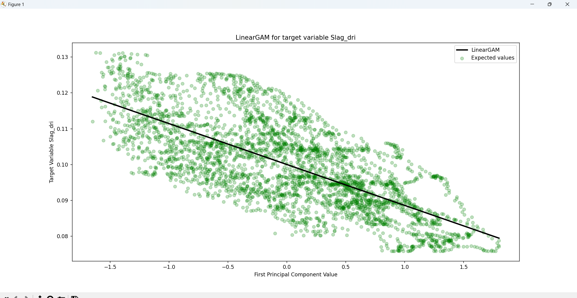
STEP 6: Model Building and Training

As mentioned before, the General Additive Model (GAM) regression model serves as a way to estimate the relationships between the dependent variables of the DR process and the independent variables that represent the qualities of the output obtained by the process. GAM is a generalized linear model which formulates a linear response depending on multiple smooth functions (which for the case of this problem are splines).

When combined with PCA, GAM can efficiently handle high-dimensional data by using the principal components as input features which are then adapted into individual smoothing splines (regression splines involve dividing the range of the PCA component into K distinct regions where a polynomial function is then applied.

The GAM model for this project adapts the following form s(0) + s(1) + ... + s(5), where all 6 main PCA components are molded into smoothing splines. The GAM model is then adapted to handle all 9 dependent variables that represent the Direct Iron Ore that is generated by the manufacturing process. This is done by fitting a separate GAM model for each target variable using the selected principal components as input.

For this reason, are scatter plots the best option for visually comparing the actual observed values (represented by the scatter points) with the predicted values generated by the GAM model (represented by the line plot). This comparison helps in evaluating how well the model fits the data and captures the underlying patterns.

NOTE: By comparing the values of the first Principal Component, we can capture the most significant patterns or variations in the data between the main patterns in the data and the target variable.

Now that the (Quality prediction) model is complete, it's time to use the Reverse Stepwise Regression in order to determine the main 6 variables that will later be used for the same structured GAM model made for the Principal Components.

This can be done with the statsmodel library, which applies regression by fitting all of the variables and then measuring their respective p-values. Once the p-values have been calculated, the variable with the lowest p-value is then removed and the process starts all over again.

STEP 7: Model Evaluation and Comparison

The GCV values indicate a notable difference in predictive error, with the PCA model achieving a minimal value of 0.0001, suggesting an extremely low prediction error. In contrast, the Reverse Stepwise Regression model shows a GCV of 0.0, which might imply overfitting.

When examining the AIC values and Pseudo R-Squared values, PCA model achieves a better balance of fit and complexity by showing a significantly lower AIC and achieves a Pseudo R-Squared of 0.3382, suggesting that about 33.82% of the variability in the outcome can be explained by this model. Conversely, the Reverse Stepwise Regression model boasts a much higher Pseudo R-Squared of 0.8252.

In conclusion, while the Reverse Stepwise Regression model excels in explanatory power as reflected by its high Pseudo R-Squared value, the PCA model demonstrates better overall performance when considering the balance of prediction accuracy and model simplicity, as indicated by its lower AIC.

STEP 8: Model Refinement

By comparing the result of the GAM models that use PCA with the models that use only the statistically relevant variables obtained from the Reverse Stepwise Reduction technique, we can see that even though both are mathematical techniques specialized for dimension reduction, there is considerably more value lost in one technique than the other.

Some aspects that we have to value from the PCA models are their inherent ability to enhance the performance of the GAM models in a way where there is no value lost that would otherwise be discarded from the reverse stepwise regression technique.

At the end of the day, even though one model offers a better fit than the other, we should always consider the computational costs that arise when handling with large quantities of features (which is extremely common in a manufacturing process).

Conclusion:
The use of GAM models in manufacturing processes like Direct Reduction could bring plenty of value in the reduction of waste (Quality Control) and the forecasting of end results (Quality Prediction), thanks to the insights obtained from the analysis of PRINCIPAL COMPONENTS and/or STATISTICALLY RELEVANT variables.

This insight facilitates root cause analysis and enables targeted interventions to improve the performance of the process and the quality of it's final product. All thanks to the examination of the estimated coefficients and smooth functions in the GAM model, manufacturers can pinpoint which variables have the most significant impact on product quality and how they interact with one another.